Detailed Info on How to Use a Tektronix 465 Oscilloscope:

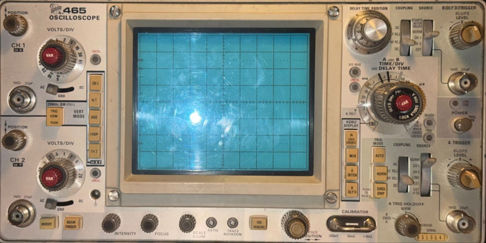
This post helps to go through the basic functions and additional measurements you can do with the Tektronix 465 Oscilloscope. Through feedback and surveys, this post will be updated to include more complex functions and questions on how to use this device for a requested activity. If there are any questions, please refer to the following sources below and if they are not answered, please feel free to comment below the last video of our YouTube tutorial.

This oscilloscope guide does not include the DM44 function as scene in most manuals.

This tutorial can be used for an older function generator, but when calibrating and learning, please use with a known working function generator so you can see the base workings and offsets of your oscilloscope. After knowing that your device works properly or improperly, you can then make accurate measurements based on your known working measurements.

[TOC]

Equipment

The equipment below is required for testing and using the oscilloscope, as well as circuits.

• 50 ohm feedthrough adapter

• 2-3 BNC cables

• BNC tee adapter

• BNC Test adapter

• Known working multimeter

• Known working function generator

Screen Handling and Setting Up

Basic Controls

An oscilloscope has a few controls that help with scaling and moving the signal to fit within the viewing window.

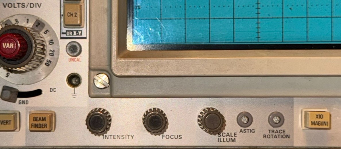
INTENSITY changes how bright the signal appears. Keep this generally the same level, unless using A and B TIME/DIV measurements. This might have to be fiddled with according to how bright the B gate is. In general, keep the brightness at an even slightly dim level in order not to permanently burn the phosphorus screen. Many pictures shown in this tutorial are purposefully brightened to show the wave form.

FOCUS is for when you are changing the size and scale of your signal. This might have to be changed as you change your signal.

SCALE ILLUM brightness the graticule brightness and the black grid lines. These turn orange when brightened. This function is really only used in dark spaces.

ASTIG permanently adjusts focus. This is usually something you may have to adjust once and never again. It should be used with the focus setting, but does not need to be adjusted frequently.

TRACE ROTATION adjusts the trace of your wave to align with you graticule lines. This also is rarely adjusted.

Screen Units

Within an oscilloscope, there are lines called graticules that show the devices measurement system. Each box, or graticule section, represents one division, or “DIV” on most buttons/dials. For instance, when using CH1 or CH 2 VOLTS/DIV dials, each vertical deflection will show approximately the highlighted amount of volts PER graticule. If the oscilloscope is properly receiving 2 V into one channel and your dial is set to 1 VOLTS/DIV, then your wave, when centered, should span across 2 graticules, the top and bottom of the wave touching the top and bottom line of that graticule. See Peak to Peak Measurements if you want to know how to measure the full frequency of the wave.

Channels

Channels 1 and 2 are the main inputs for measuring waves with this oscilloscope. Channel one should be the main terminal used, and is the main terminal used in this guide. When comparing two signals, Channel 1 is often used as the main signal to be measured, and Channel 2 is the steady reference signal. For the X-Y display, Channel 1 or X is the horizontal deflection, and Channel 2 or Y is the vertical deflection.

---

Checks

Calibrating Probes

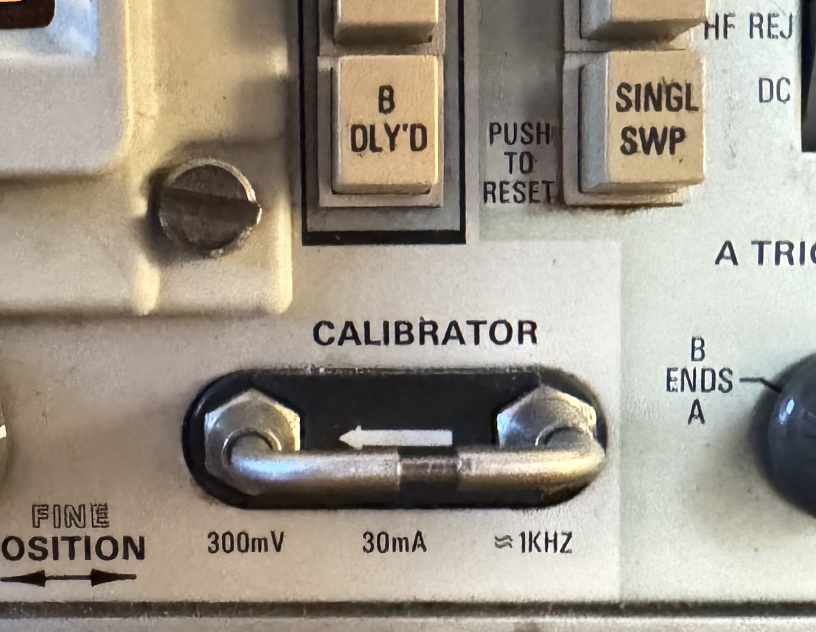
The calibrator is the metal rectangle probing out at the bottom right of your oscilloscope. Your first step when receiving your oscilloscope and probes is to calibrate these probes using the calibrator. You should have 1-2 probes for this device. Label your probes for channel 1 and channel 2, and use as accordingly.

1. Connect your probe to its corresponding channel. You can do this one at a time, or both at once. For one at a time, select Vert Mode to the corresponding channel you are using, and for doing both, press the ALT mode. Use the POSITION dial of either channel to accurately place the functions into view. Calibrating your probes one at a time will help you more accurately adjust the traces.
2. To denoise the wave, take a banana clip and attach a wire to the end of it so you can clip your grounding clip to it. Plug the banana clip into the grounding hole below the vert mode buttons.
3. Clip your probe onto the middle of the calibrator bar.

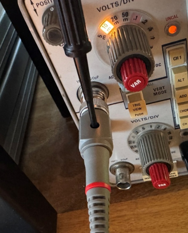
Below is what your set up should look like:

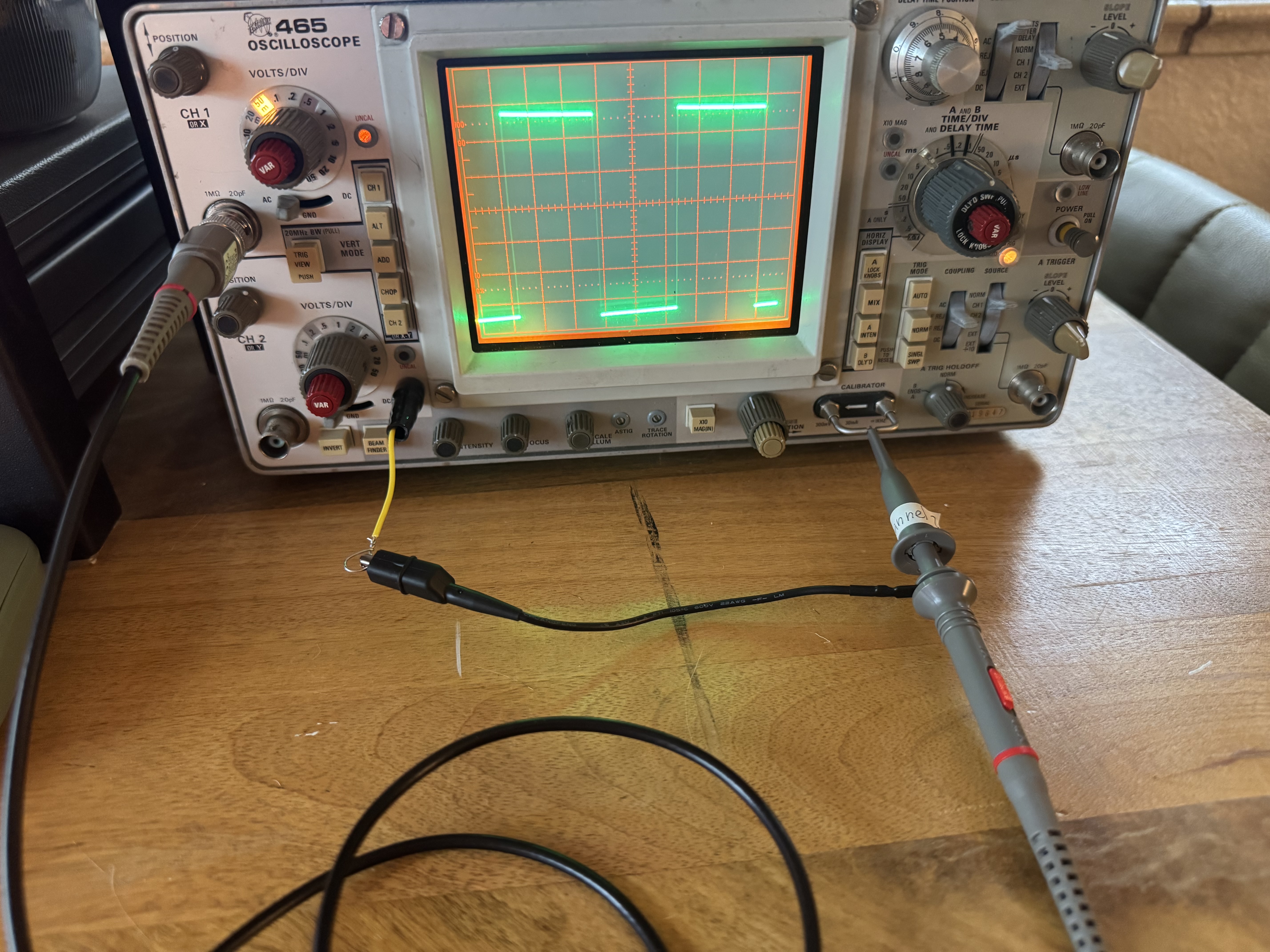
You should see a display on your screen that may or may look as curved as the one down below. If your screen looks like either of the pictures below, you need to calibrate your probe.

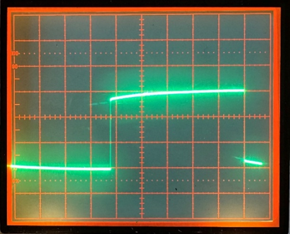
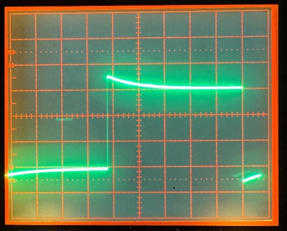
On the back of the probe should be a hole with a set screw. Turn that knob until the square waveform is the straightest that it can be. It should look like the picture below.

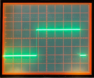
After this, do the same for Channel 2 with the second probe. You have calibrated your probes! You want to keep one probe per channel as the channel input of each can be slightly different, and your probes will stay consistent.

Vertical and Horizontal Check

A vertical and horizontal check will ensure your device in reading waves in a precise manner.

Vertical Check:

1. Hook up your probe to the square wave calibrator bar as seen in the previous example.

2. Set VOLTS/DIV to the 50 mV position and the input coupling switch to DC.

3. VAR VOLTS/DIV, the small red dial on the VOLTS/DIV knob, should be in the calibrated indent, the UNCAL lamp should be off. The vertical deflection should be between 5.8 to 6.2 division. If not, you can either fix the interior, or adjust the VAR VOLTS/DIV to adjust for the proper measurement.

Horizontal check:

1. Obtain a Normal Display.
2. Set the A TIME/DIV switch to 5 ms position. Set the A Trigger SOURCE switch to LINE.
3. Push the TRIG VIEW switch and hold it in. This displays a sample of the line voltage.
4. Use the A Trigger LEVEL control to vertically position the top of the display to with in the display area.
5. Use the horizontal position control to position the left peak to the left graticule edge. Verify the horizontal distance between the first and the fourth peaks is 9.8 to 10.2 divisions. If the fourth peak is not visible, verify the horizontal distance between the first and the third peaks is 6.53 to 6.79 divisions.

Basic Use

Displays

Normal Sweep Display

Normal Sweep Display will commonly be referred to as the baseline display.

Vertical Section:

Vert Mode: Set to Channel 1

VOLTS/DIV: Adjust for input amplitude

VAR VOLTS/DIV: Calibrated, UNCAL lamp off

AC-GND-DC: AC

POSITION Vertical: Mid position

INVERT: Button Out

Horizontal Section:

TIME/DIV switches: locked together at 1 ms

VAR TIME/DIV: Calibrated Detent

HORIZ DISPLAY: A

X10 MAG: Off

POSITION Horizontal: Midrange

Trigger:

SLOPE (click dial): +

LEVEL(turn dial): 0

SOURCE: NORM

COUPLING: AC

TRIG MODE: AUTO

A TRIG HOLDHOFF: NORM

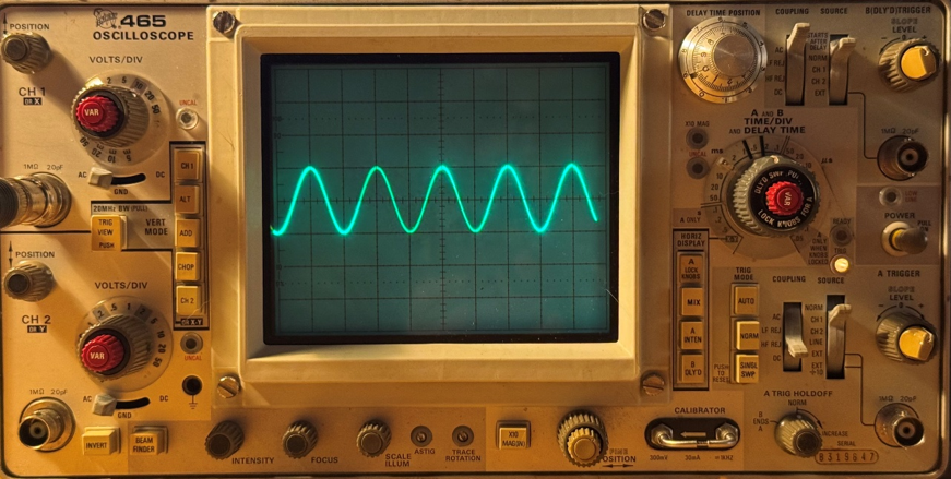
Delayed Sweep Display

1. Normal Sweep Display
2. Set HORIZ DISPLAY switch to A INTEN and the B trigger SOURCE switch to STARTS AFTER DELAY
3. Pull on B TIME/DIV know and turn cw until the intensified zone is the desire length. Adjust INTENSITY for desired brightness.
4. Adjust DELAY TIME POSITION control to move intensified zone to cover portion of the display to be displayed in delayed form.
5. Set HORIZ DISPLAY switch to B DLY’D. Delay sweep is indicated on the B TIME/DIV knob.
6. For less jitter, set B trigger SOURCE switch to the same position as the A trigger SOURCE switch and adjust the B LEVEL control for a stable display.

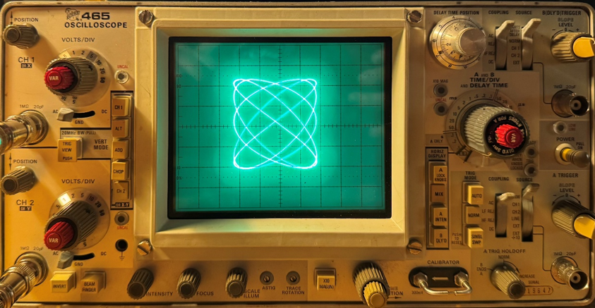
X-Y Display

1. Step one of Normal Sweep Display
2. Set the TIME/DIV switch to X-Y and the VERT MODE button to CH 2. Apply the vertical signal to the CH 2 OR Y input connector and the horizontal signal to the CH 1 OR X input connector.
3. Use intensity to the find beam, if not shown, hold down beam finder and adjust the CH 1 or CH2 VOLTS/DIV until display is reduce in size. Release beam finder and adjust focus for clearer picture.

AC, GND, and DC

AC, GND, and DC is the mode used to couple the input signal to the vertical amplifier. This basically means that depending on which mode you use, you are sending certain parts of the vertical part of the inputting signal to the oscilloscope.

Alternate Coupling (AC): The fluctuation of the current

Direct Coupling (DC): Offset of the current

If you set an offset to you current in a function generator and have you oscilloscope set to DC, you will see the waveform and offset. If it is only set to AC, you will only see the waveform as the device cuts off the DC coupling. Ground isolates both of these functions and you will simply see a line. This can be useful is you want to see the 0 V offset, where the middle or 0 trace of your waveform will be.

ADD Mode

The ADD function of VERT MODE displays the algebraic sum of the signals applied to Channel 1 and Channel 2 inputs. This function is helpful for testing and analyzing waves that combine in an circuit. It is also helpful for seeing if two waves are simultaneous, contain wave delay, and if there is any visible distortion in either signal.

Before using this function, there are a few things to keep in mind to use the function properly.

1. Not not exceed the input voltage rating of the oscilloscope. This can damage internal parts, and can permanently mess up readings. To avoid this, use a lower voltage or use a probe that can divide your signal voltage by 10.
2. Do not apply signals that exceed an equivalent voltage of about 8 times the VOLTS/DIV switch setting used. For instance, if you are using a VOLTS/DIV switch setting of 0.5, the voltage applied to the channel should not exceed 4 volts. This can distort the display and possibly overload the oscilloscope.

When using the ADD mode, inverting Channel 2 can either add up your signals, or work slightly as a “subtract” function. If your signals match each other, inverting channel 2 can help you see any discrepancies within the added signals. If Channel 2 is inverted from Channel 1, the inverted button can help correct this without changing the wave.

You can also use the ADD mode to provide a DC offset for an AC signal. For example, if Channel 1 is an AC signal, use Channel 2 to apply a negative DC offset, then apply the ADD function to add this offset together. This is helpful when you cant adjust the position of a signal.

Triggering

Triggering is meant to synchronize your waveform every time it samples. For digital oscilloscopes, there are many “automatic” triggering functions that make it very easy to automatically synchronize your waveform without much input. Analogue oscilloscopes are far more manual. The oscilloscope has three trigger functions.

AUTO mode: The sweep is initiated by the applied trigger signal, however in the absence of one or if the trigger in less than 20 hertz, the sweep free runs and gives a bright reference trace of the input signal.

NORM mode: This mode only shows the trace only when the adequate trigger if found. Use for steady traces or when the trigger rate is too low for AUTO mode.

SINGL SWP: This mode is meant to display a single sweep of the signal only when the button is pushed. This mode is mainly used to look at and photograph non-repetitive signals.

The Channel 1 and Channel 2 trigger inputs allow for external trigger signals. Triggered and untriggered examples below.

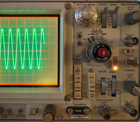
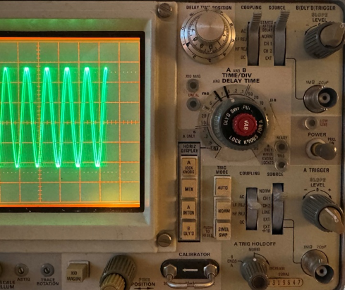
The triggering knob is labeled with a “Slope Level [- 0 +]”. This indicates the slope the trigger signal starts on. The “Slope” part of the knob is the knob that clicks to either the negative sign or the plus sign. The “Level” part of the knob indicate where on the wave the trigger will trigger at. Keeping this at 0 for basic set ups is the most common use, and will keep the trigger line in the center of the horizontal part of the wave.

The A sweep is the default signal to change, measure, and trigger your signals, thus use the A trigger knob . A - B trigger and delay will be detailed more below in the A and B

Voltage Measurements

Peak to Peak Voltage - AC

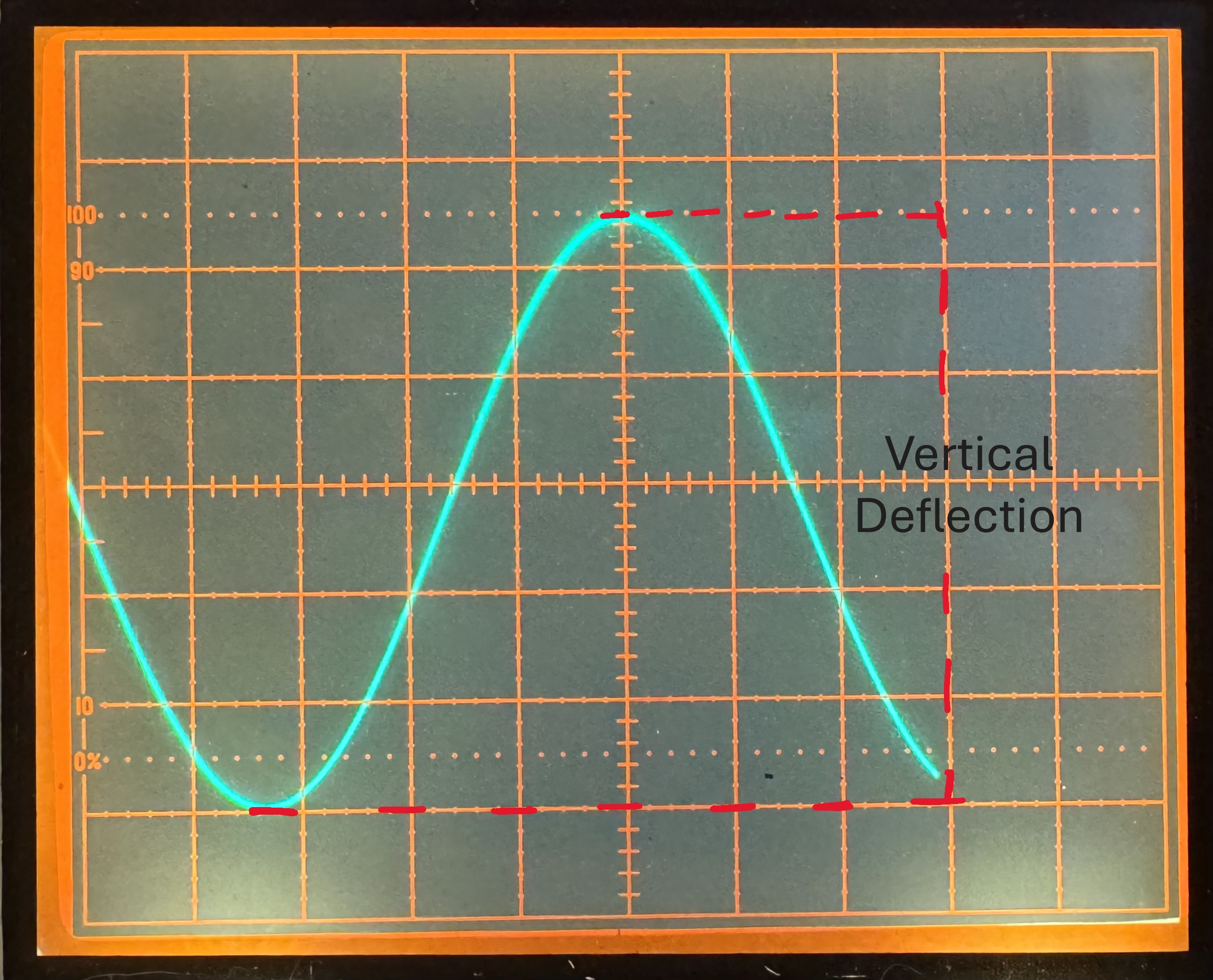
To measure peak to peak voltage, obtain a normal sweep display of a voltage of your choosing, and line the highest peak of your wave with the center vertical graticule line. Next align the the closest lower peak with a horizontal graticule line. The “vertical deflection” is the amount of graticules the vertical aspect or your wave takes up. Multiply the vertical deflection by your VOLTS/DIV setting, resulting in your peak to peak voltage.

In the example below, the wave has a vertical deflection of 5.5, with a VOLTS/DIV setting of 20 m.

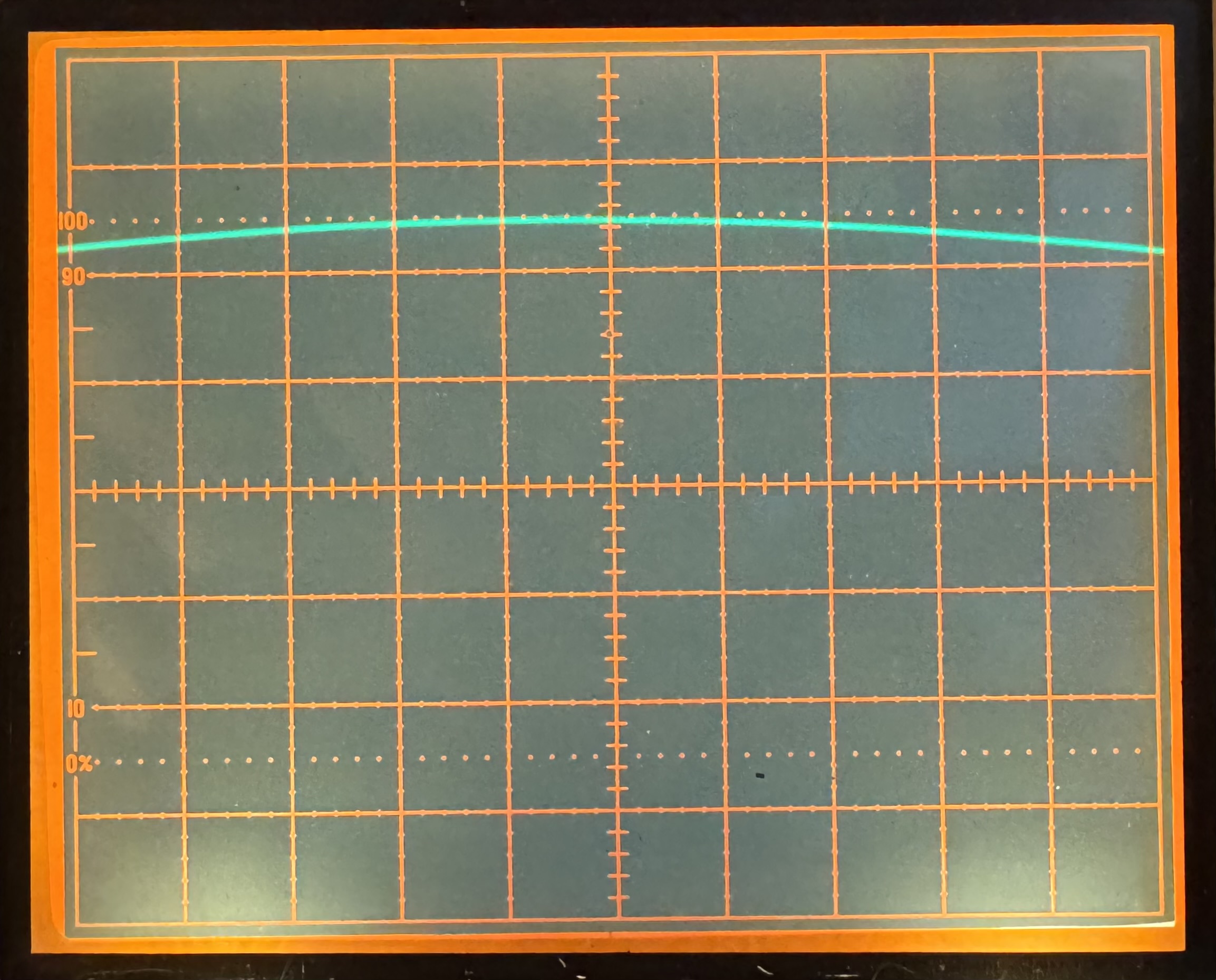
With the the X10 MAG button, you can see a more accurate display of the top of your wave form. In this example, it confirms our wave is right between the markers.

Instantaneous Voltage Measurement - DC

To find the instantaneous voltage, start with finding the polarity. To find the polarity, obtain a normal display and set input coupling to GND. Vertically position the line to the center of the CRT display then set the coupling to DC. If you see the point on you line move above the center line, the voltage is positive,if below the center, the voltage is negative.

To find the voltage value, first switch input coupling to GND. If you had a positive voltage, position your line to a bottom reference graticule, and if it’s negative position your line to reference in the positive graticule. The example below showed a positive voltage so it should be positions as such:

Next switch your coupling switch to DC. If your voltage is positive, measure the vertical deflection, which is the divisions between the bottom of the screen and your point being measured on the wave. If your voltage is negative, the vertical deflection will be measured from the top of the screen, to your reference point. IN the example below, the measurement was taken from the bottom graticule to the top reference point.

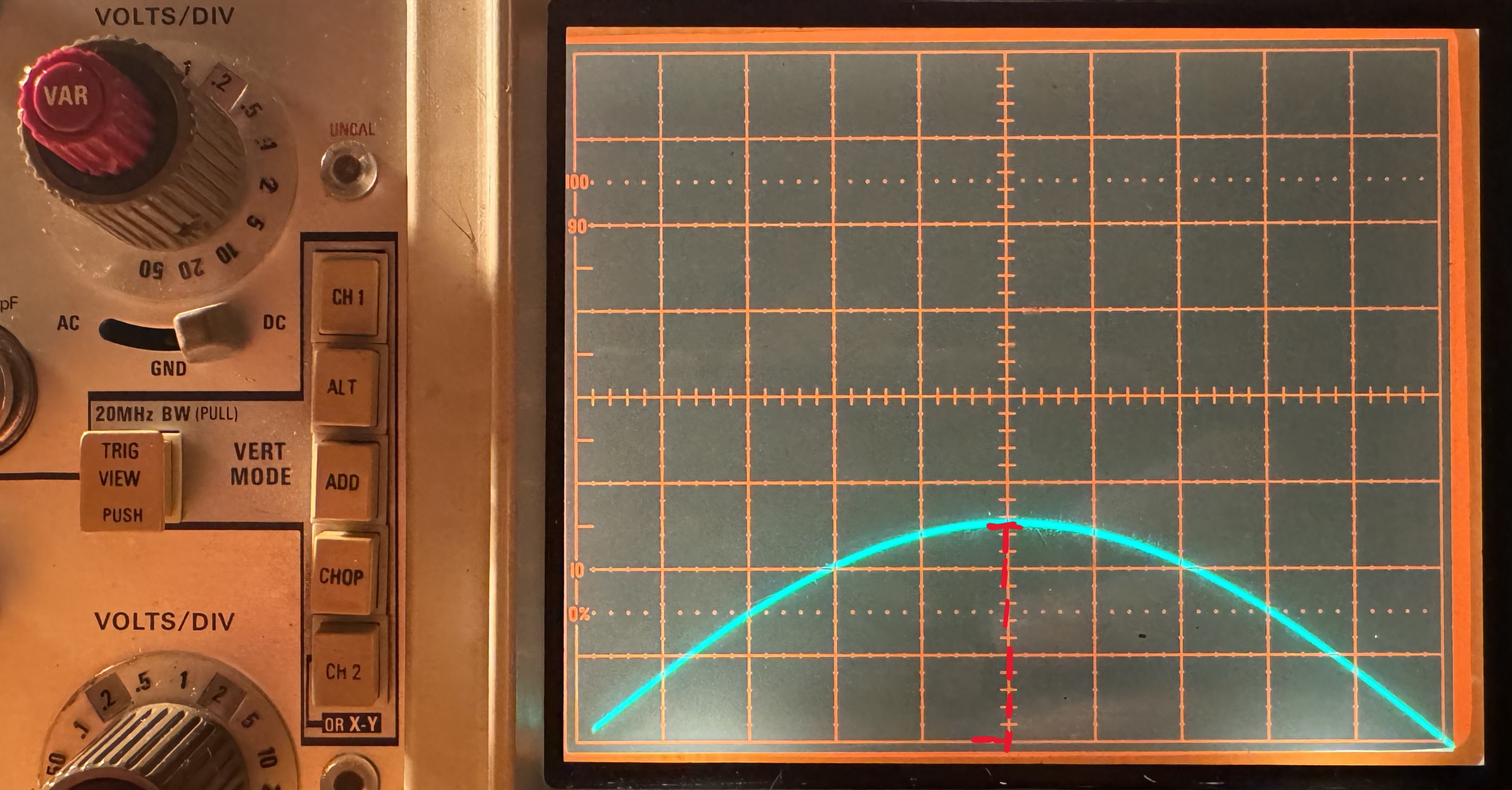
Multiply the vertical deflection by the VOLTS/DIV switch setting to achieve your instantaneous voltage. In this example, the VOLTS/DIV setting is set to 20 mV.

Time Measurements

Time Duration Measurements

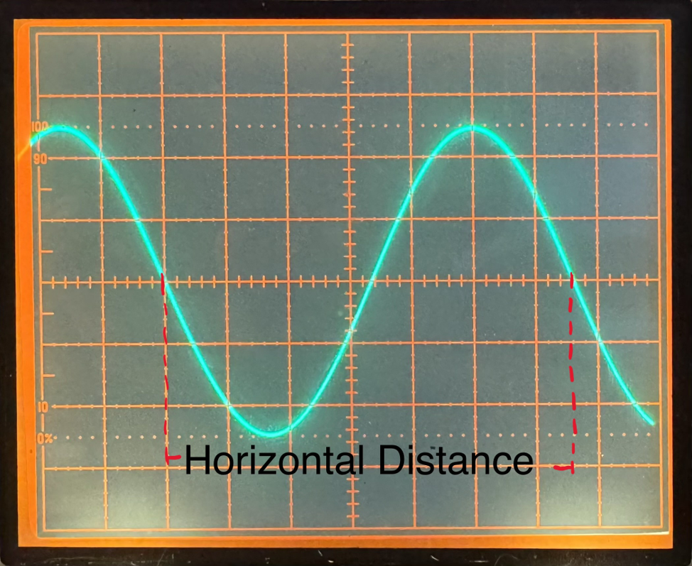
To measure the time duration obtain a normal sweep display of a voltage of your choosing. Center the wave vertically and set the time/div position to enable a single wave as wide as possible visible on the screen. Measure the horizontal distance between the two points where the wave starts and ends. It helps to center your first point of measurement on a graticule line to get a more accurate value. Multiple this measurement by the time/div switch value. If you are using the X10 button, divide the resulting value by 10.

For example, this wave measures roughly 6.6 graticule lines, and the TIME/DIV switch is set to 50 microseconds, so the time duration is roughly 330 microseconds.

To obtain frequency measurements from time duration, and divide 1 by your result.

The example above shows a time duration of roughly 330 microseconds, or 0.00033 seconds.

Time Difference Between Two Pulses Measurements from Different Sources:

This method makes sure that both pulse time delays are accurate.

Obtain a normal sweep display for both pulses and center them both so they are overlapping. Connect the reference signal to channel 1 and the comparison signal to channel 2. Set the vert mode switch to CHOP for low-frequency signals, and use alt for higher frequency signals. Set the A trigger source to NORM, and set the A trigger SLOPE to either positive or negative, and the A trigger LEVEL to just under 0.

If one of your waves is “running” when switching to channel 1 on the A trigger SOURCE, you can sync your trigger by connecting a BNC cable to the SYNC output on both of your funciton generators.

Make sure both pulses are of equal frequency and time delay. You can make your reference pulse 50% of your comparison pules for better visualization, however in the example below, both are of equal amplitude.

Since you are finding the time distance between two points, the time difference equation is the same equations as the time duration equation. To obtain this, measure the horizontal difference between both pulses, and divide this distance by the time/div switch.

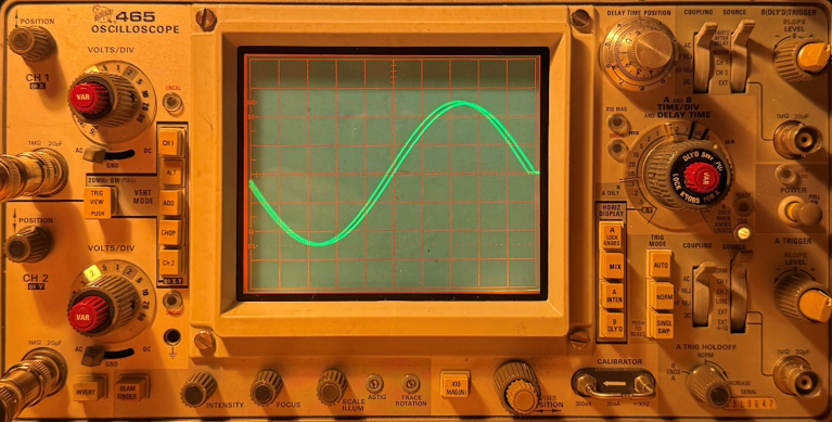
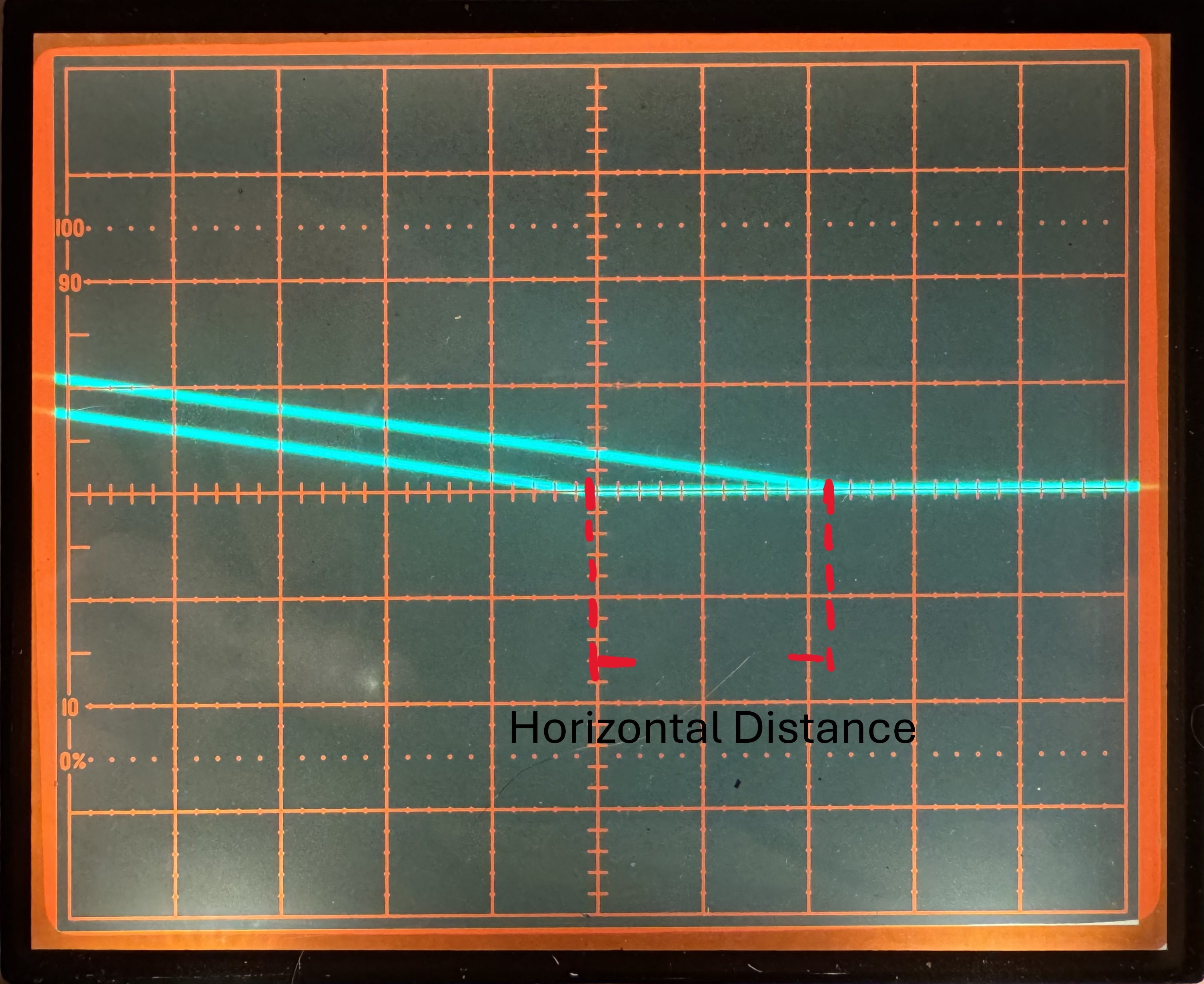
For the example below, we will be using the X10 mag button. We measure 2.2 graticules for the horizontal distance, 50 microsecond as our time div. The result will be divided by 10 since the X10 button is being used. We obtain the following measurement:

Rise Time Measurements

Risetime measurements use the 10% and 90% graticule lines on the screen.

Obtain a normal sweep display, and set the A slope to +. Set the VOLTS/DIV setting to 5 divisions, and the TIME/DIV setting to display multiple cycles so you can see the top and bottom of all cycles. Vertically position the wave so that the bottom of the entire wave touches the 0% dotted graticule line, and the top of the entire wave touches the 100% dotted graticule line.

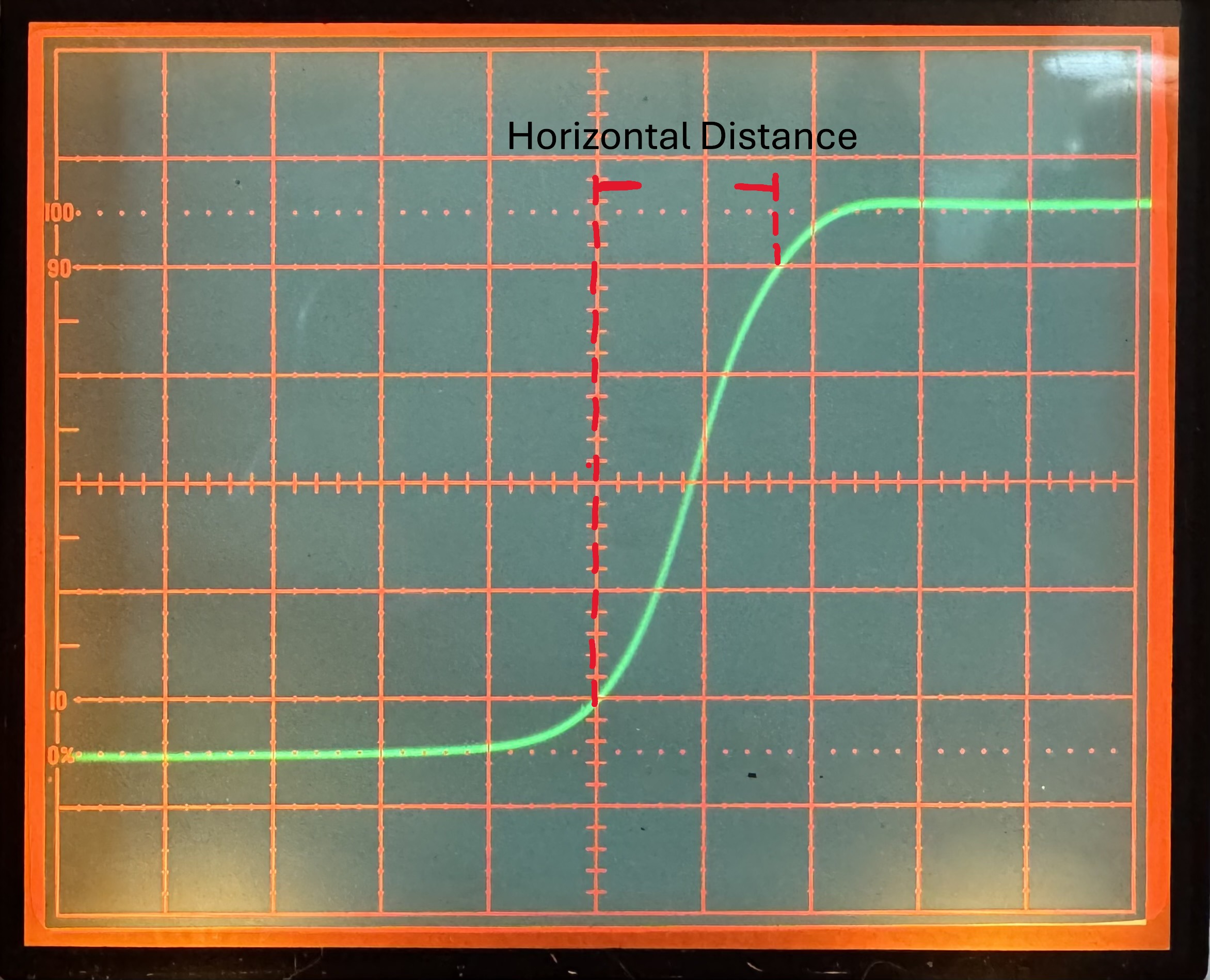
Next, Change the TIME/DIV setting to as wide of a setting that can be managed, for the example below with a square wave of about 9k Hz in frequency and and amplitude of 1 V, 0.05 and 0.1 microseconds works fine. Measure the distance between where the wave hits the 10% and 90% graticule lines. It helps to line up one point with your center or a chosen graticule line. This will give you the total risetime.

In the example below, I am using a square wave on 9k Hz and 1 V. My TIME/DIV setting is set to 0.05 microseconds. This example is also using the X10 mag button for better resolution.

Phase Difference

Measuring the phase difference is similar to finding the time difference, however it takes into account the phase based on how many graticules a full wave cycle spans.

First, use CHOP or ALT mode, and set the A TRIGGER SOURCE switch to CH 1. Use coaxial cables that have equal time delay to connect the signals to the input connectors. If the signals are opposite in polarity, use the INVERT pushbutton to invert the Channel 2 display. Set CH 1 and CH 2 VOLTS/DIV switch and the CH 1 and CH 2 VAR controls so the displays are equal in amplitude. It does not matter if either are properly calibrated as the horizontal measurement is the desired value, not the amplitude.

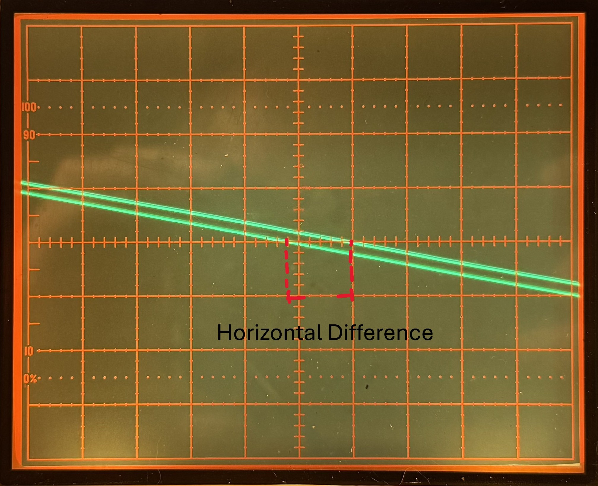
Set TIME/DIV switch so that your wave span about eight of ten graticule. The example below shows 1 full cycle across eight divisions which will give a sweep rate of 45 degrees/division. This is because one cycle will span 360 egree, and 360 devided by 8 is 45. If you are spanning your waves across ten divisions, you should calculate your answers with 35 degrees/division. Theoretically, a cycle spanning any number of division will work with the applied degree/division calculation, but 8-10 graticules will provide a more accurate measurement. The two points being measured is one one at the left edge of the negative 4th graticule, and one on the right edge of the positive 4th graticule.

Measure the horizontal difference between two corresponding points on the waveform and multiply the distance measured (in divisions) by 45 degrees/division (sweep rate) to obtain the amount of phase difference.

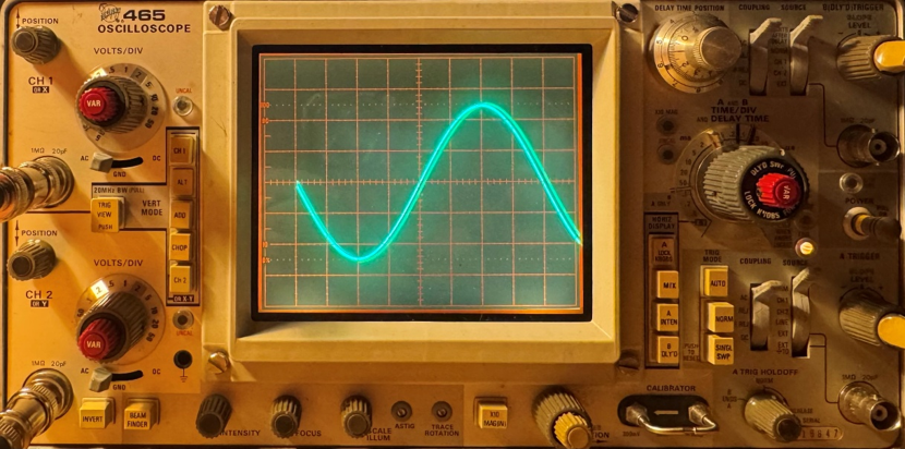
Simply observing the wave like this will probably not give you an accurate measurement, so use the X10 magnification button to obtain a more accurate display. If using this method, make sure to divide the resulting sweep rate shown by 10.

In the example below, the cycle spans 8 divisions (45 degrees per division), and has an X10 magnification measurement of 1.2 graticules.

A and B Time Delay

The A and B time delay knob is very useful to measure your wave, create separate triggers, and affect one wave with another. For most of your initial measurements, you have been using the A TIME/DIV delay options. The B sweep is an added function to delay your initial A sweep. Both sweeps have COUPLING, SOURCE, and TRIGGER controls.

Mixed Sweep Display

First, familiarize yourself with the Mixed Sweep Display.

1. Normal Sweep Display
2. Pullout on the B TIME/DIV knob and turn CW to the desired sweep rate
3. Set HORIZ DISPLAY switch to MIX. The display now contains two sweep rates. First portions of display is at the A sweep rate while the later portion of the display is at the B sweep rate. The start of the B sweep rate portion can be changed by adjusting the DELAY TIME POSITION control.

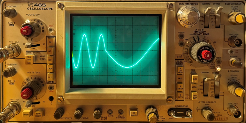
You can also use this function to use Channel 2 frequency as a trigger. To do this, switch A trigger SOURCE to Channel 1, and trigger the LEVEL. Switch B trigger SOURCE to channel 2 and trigger the LEVEL to where you see a moving wave.

To start, down below are the A and B time delays, the first one untriggered and the second one is triggered.

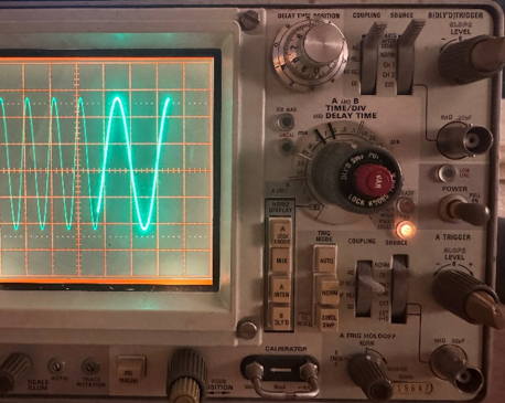
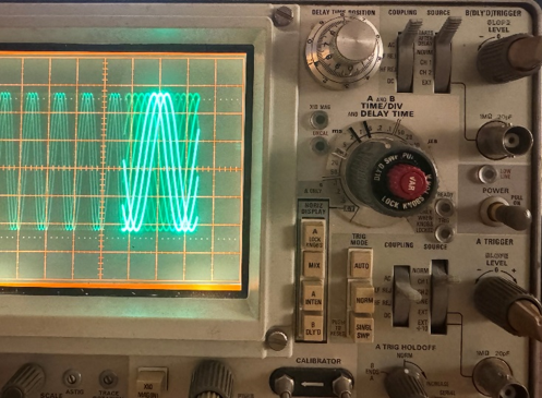
You can use this basic function to zoom in on portions of your wave, especially paired with the X10 MAG button.

If you set B trigger SOURCE to NORM, you can use the DELAY TIME POSITION dial to display segments of the wave. Using the A trigger LEVEL, and the B trigger LEVEL, you can set where your wave segment triggers. The A trigger LEVEL control the right side of the B trigger, and the B trigger LEVEL controls the left side of the B trigger.

Magnified sweep starts after delay

The magnified sweep starts after delay function allows you to zoom in on your wave form in a more precises way than that would previously been seen with the X10 mag button. This function allows you to choose the part of your wave you want to zoom in on with the delay time position dial, using the B delay function.

1. Start with a normal sweep display.
2. Set VERT mode to whichever channel you are using, and set the VOLTS/DIV to produce a display about 4-5 divisions in amplitude.
3. Making sure HORIZ DISPLAY is set to A LOCK, shorten your A time delay so you display 1-2 complete waveforms.
4. Now, set the HORIZ DISPLAY switch to A INTEN. Switch your B trigger SOURCE to “STARTS AFTER DELAY”, and B trigger COUPLING to AC. Set the B trigger SLOPE to positive and the trigger LEVEL to 0.
5. If you scroll to the right end of your wave, you will see a highlighted portion of your wave. Use the DELAY TIME POSITION dial to select the portion of your wave you want to zoom in on.
6. Pull out on the TIME/DIV main dial and rotate to the right. This is the B time delay dial, pulling out unlocks the B delay function. On the A INTEN horiz display, you can see the highlighted portion become smaller the more you rotate this to the right.
7. To view your wave, set your HORIZ display to either MIX or B OLY’D. Mix allows you to view your main wave with the highlighted portion expanded to the delay you have selected. B DLY’D allows you to view jus the highlighted portion.
8. Time measurements can be made as listed above. Just make sure to use the correct sweep rate when calculating. Amplitude measurements are made the same as stated above.
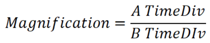
9. To find the magnification rate, divide the A TIME/DIV setting by the B TIME/DIV setting.

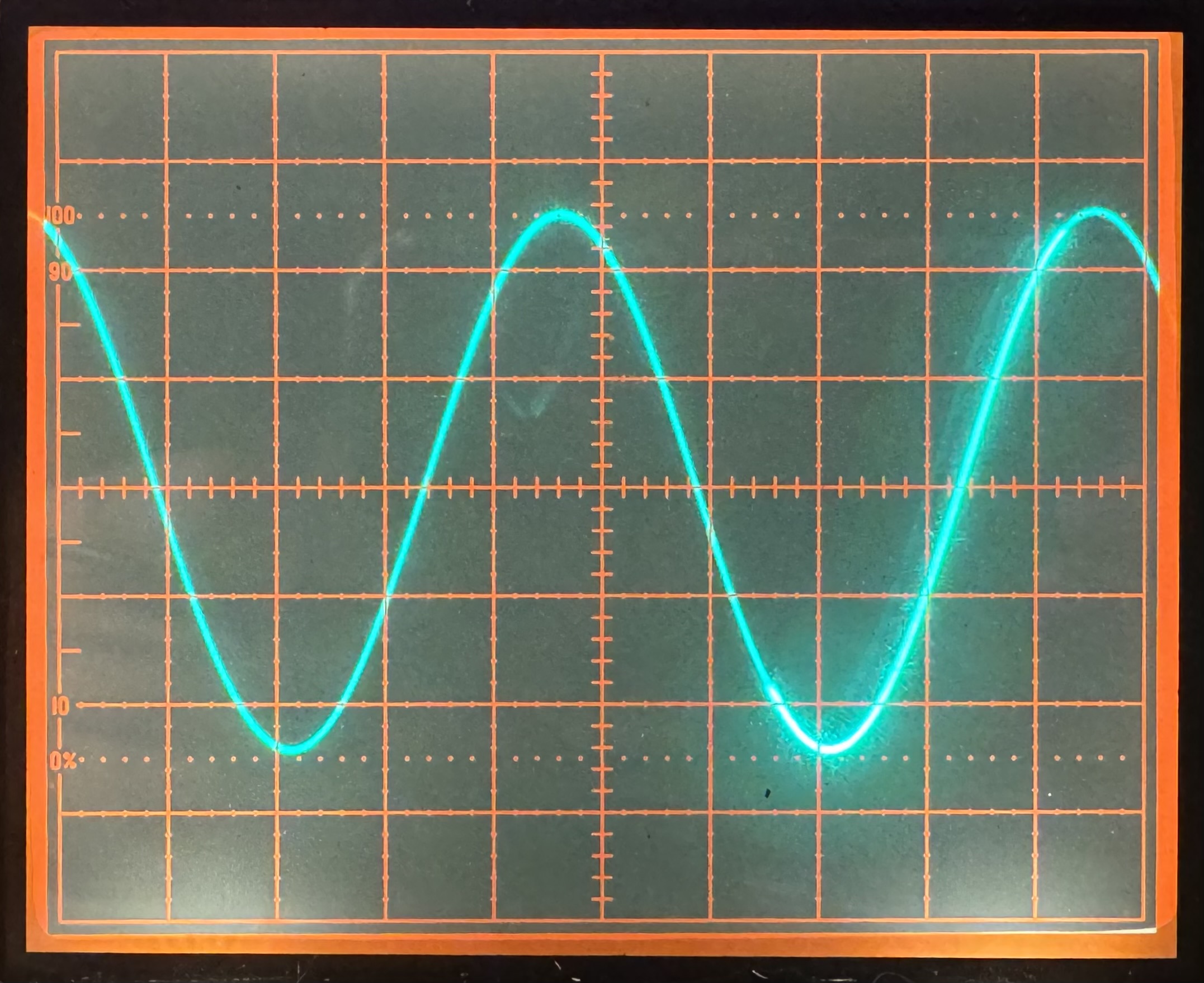
A INTEN display with 2 ms A sweep and 50 microsecond B sweep

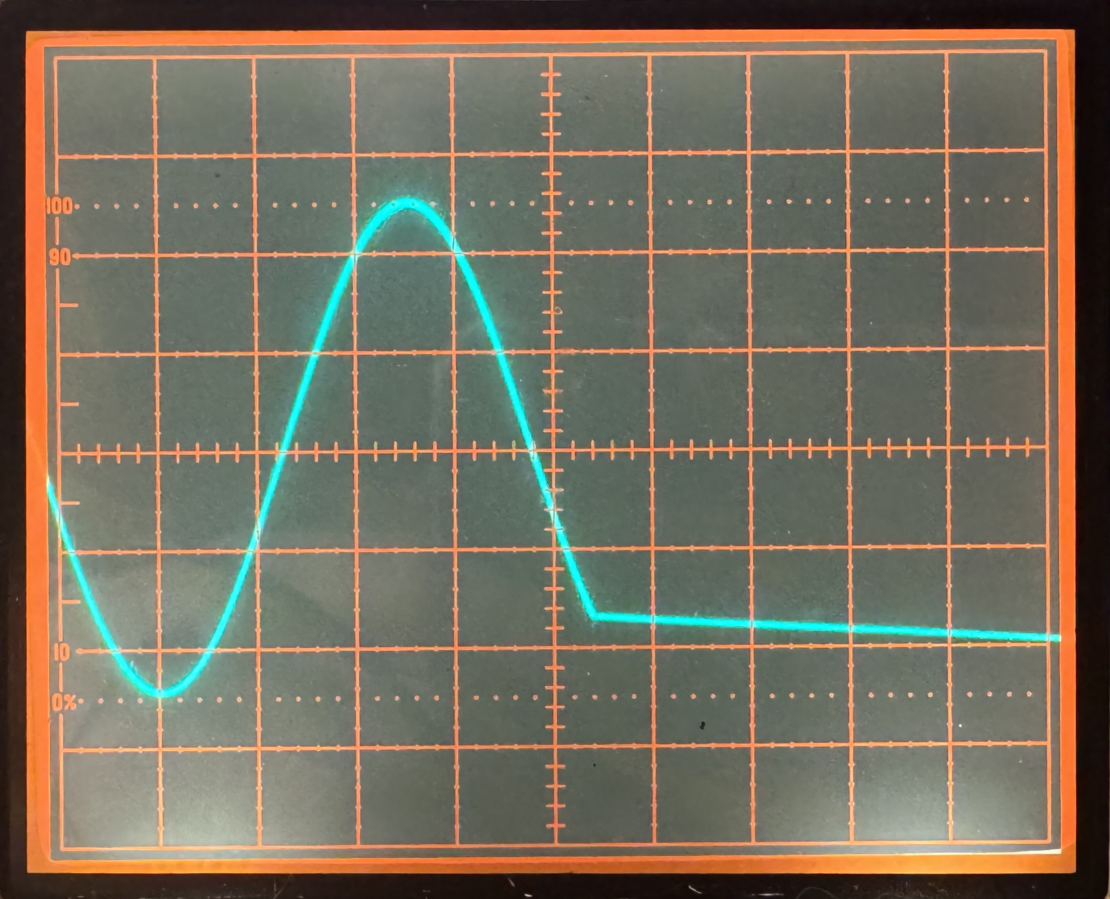
MIX Display with 2 ms A sweep and 50 microsecond B sweep

Magnification of A and B sweep in terms of seconds:

The B sweep is magnified 4 more times than the A sweep.

Triggered delayed sweep magnification

The triggered delayed sweep magnification allows you to see a far more stable wave, canceling out much of the jitter you may see with the method above.

1. Follow steps 1 through 6 on the section above.
2. Set the B trigger SOURCE to the same position as the A trigger SOURCE.
3. Adjust the B LEVEL control so the intensified zone on the trace is visible or stable. If you cannot find the highlighted zone, increase the amplitude or A TIME/DIV. Also check that you are not in X10 MAG mode. If these methods don’t work, trigger the B sweep externally.
4. Once you have the correct portion highlighted, select B DLY’D or MIX to view selected display.

All measurements made in this mode are the same as delayed sweep magnification.

Time difference between repetitive pulses

This section shows you how to use the DELAY TIME POSITION dial as a form of measurment.

1. Normal Sweep Display
2. Set the B TIM/DIV to the fastest sweep speed that vies usable intensified zones.
3. Set HORIZ DISPLAY to A INTEN and use the DELAY TIME POSITION dial to move the intensified zone to the first pulse. Note the position of the DELAY TIME POSITION dial. This will be your “First dial setting”.
4. Set the HORIZ DISPLAY switch to B DLY’D and adjust the TIME DELAY TIME POSITION dial to move the pulse to a vertical reference line. Turn the DELAY TIME POSITION dial clockwise to move the second pulse to the same vertical reference line. Note the position of the DELAY TIME POSITION dial. This will be your “Second dial setting”. Do not change the position or fine controls. If several pulses are displayed, set HORIZ DISPLAY back to A INTEN to locate the correct pulse.

The time difference is found using the following formula:

For example, below there are two square pulses. The small more highlighted dot shown is the B time delay sectioning out the rise of the first pulse. Below is a view of the pulse in A INTEN mode.

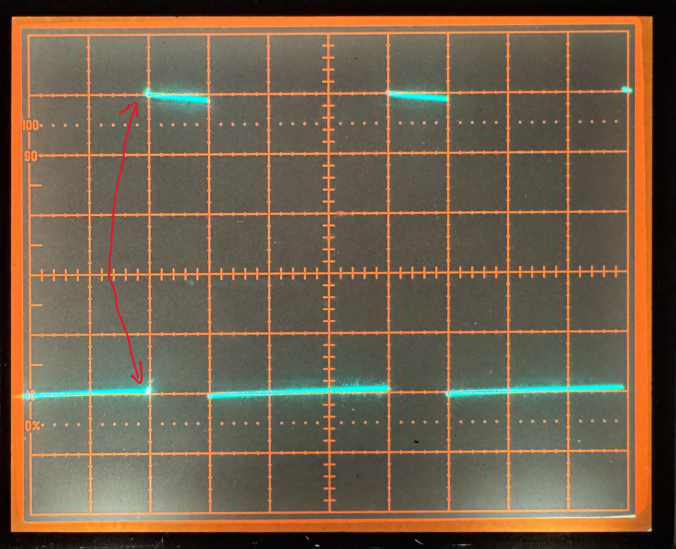
Switching to a HORIZ DISPLAY of B DLY’D and align the pulse line with some vertical reference line, as shown down below.

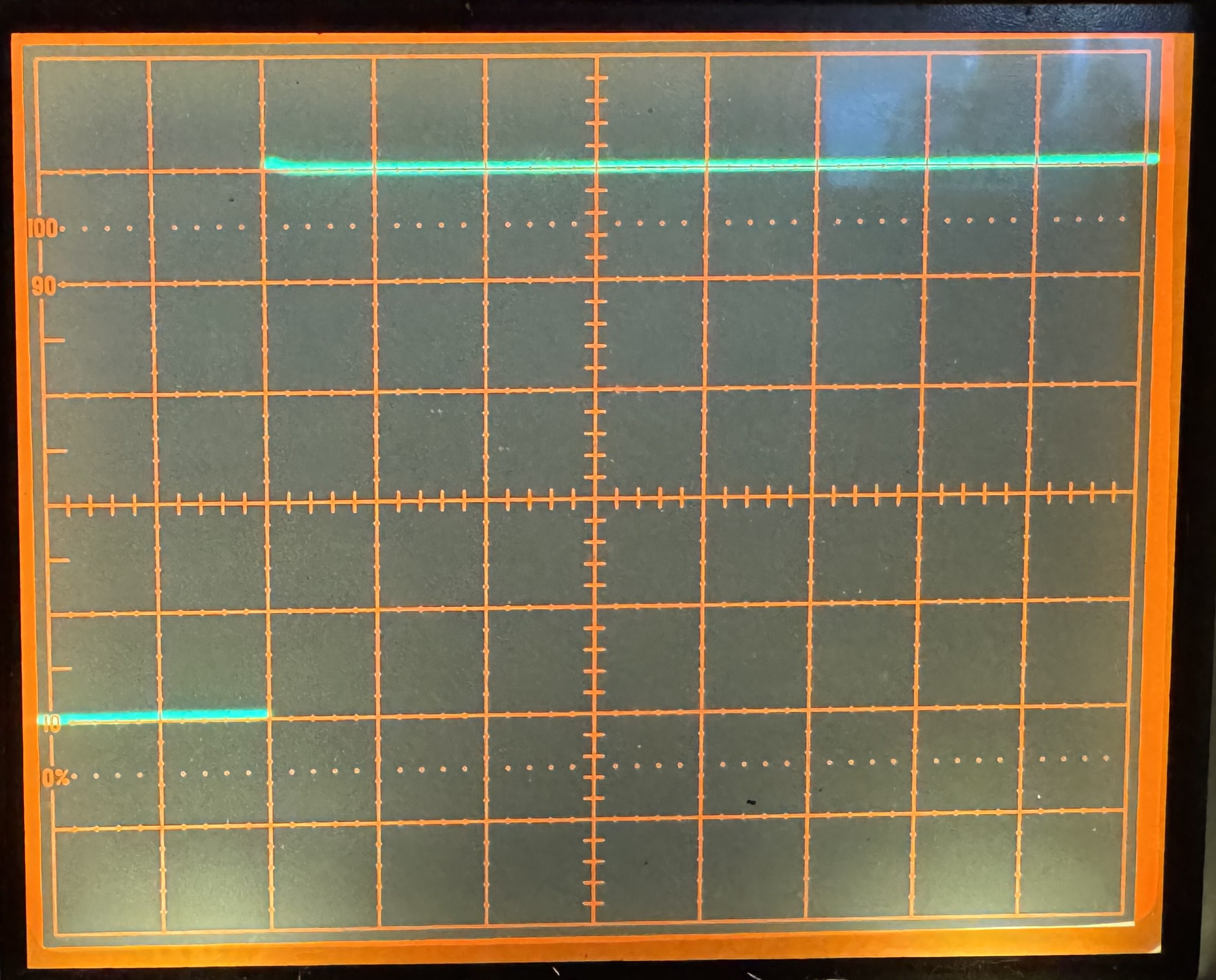
The first delay time position dial shows 3.95. Turning the dial clockwise, using the same vertical graticule line reference for the rise of the second pulse, the DELAY TIME POSITION dial shows 7.95. With an A time delay of 0.5 ms, the time difference equation gives us the following:

Appendix

Input Output connectors

Inputs

**Front Panel:**

Channel 1 (CH 1) and Channel 2 (CH 2):

Channel 1 and Channel 2 inputs are the main input connectors for the oscilloscope. When in X-Y mode, Channel 1 acts as the x connector and provides the horizontal deflection. Chanel 2 acts as the Y connector and provides the vertical deflection.

Channel 1 (CH 1) and Channel 2 (CH 2) Trigger

These inputs allow for an external trigger signals to apply to to the A or B sweep respectively.

**Rear Panel:**

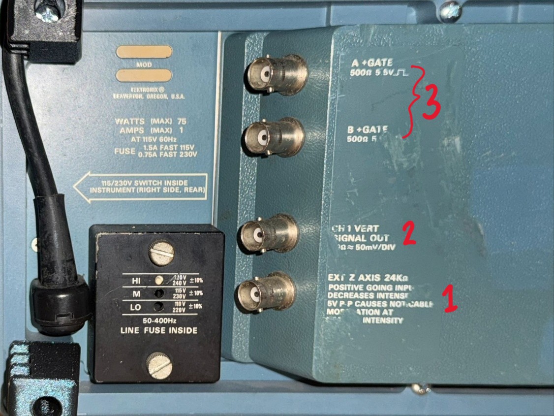
EXT Z-Axis (1):

The EXT Z-Axis input connector allows for further control and modulation of the intensity of the CRT display. Do not exceed more than 100 V plus peak for Dc or 100 V peak to peak for AC, at 1 kHz.

Outputs

**Rear Panel:**

Chanel 1 Vert Signal Out (2)

This output takes the Channel 1 signal input, and normalizes it to 50 mV per division. If you have a high voltage going into the scope, you can use this output to connect to another scope or circuit to guarantee a low or attenuated voltage for testing or safety purposes.

A + and B+ GATE (3):

This output connector provides a positive-going rectangular pulse coincident with the A sweep time and B sweep time respectively.

Controls, Connectors, and Indicators:

Vertical

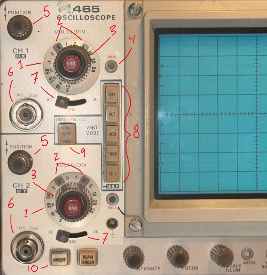
1. Ch 1 and Ch 2 VOLTS/DIV:

• Selects the vertical deflection factor in a 1-2-5 sequence (VAR control must be in the calibrated detent for the indicated deflection factor)

1. VOLTS/DIV readout:

• Two small maps for each channel. Either lamp will light up to indicate the correct deflection factor when a probe with a scale-switching connector is used. Probe without the connector lights the X1 lamp

1. VAR:

• Provides continuously variable uncalibrated deflection factors between calibrated settings of the VOLTs/DIV switch, and extends the max vertical deflection to at least 12.5 volts per division

1. UNCAL Lamp

• Indicated when the VAR VOLTS/DIV control is out of the calibrated detent and the vertical deflection factor is uncalibrated

1. POSITION:

• Positions display vertically. In x-y mode, ch2 position control positions on the y axis, horizontal positions x

1. Ch1 oR X and ch2 or Y:

• Input connectors for the application of external signals to the inputs of the vertical amplifier. In x-y mode, signal connected to ch1 of x connector is horizontal, ch2 or y is vertical

1. AC-GND-DC

• Selects the method used to couple the signal to the input of the vertical amplifier. In Ac position, signal are capacitively coupled to the vertical amplifier, dc input in blocked. In GND position, input of vertical amplifier is disconnected from input connecter and grounded to allow the input coupling capacitor to recharge. In DC position, all components of input signal are pass to input amplifier.

1. VERT MODE:

• Selects the mode of operation for the vertical amplifier system.

  • ALT: Provides dual-trace display of the signals of both channels, for sweep rates faster than 50 microsecond/division

  • ADD: Either adds of inverts signals of both ch1 and ch2. Useful for removing undesired signals.

  • CHOP: Dual-trace display of signal of both channels. Useful at sweep rates slower than 50 microsecond/division.

  • CH2: Must be selected in x-y operation

1. 20 MHz BW/Trug view:

• Limits bandwidth of vertical amplifier system to 20 MHz when pulled, and causes signal applied to A trigger generator to be displayed on CRT when pressed.

1. INVERT:

• Channel 2 display is inverted

Display

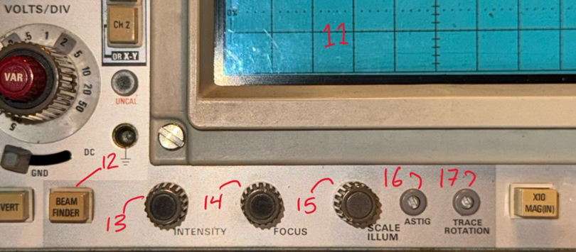
1. Internal Graticule:

• Eliminate parallax. Risetime, amplitude and measurement point are indicated at the left-hand graticule edge.

1. BEAM FINDER:

• Compresses the display to within the graticule area independently of display position or applied signals. Visible viewing level.

1. INTENSITY:

• Brightness

1. FOCUS:

• Adjust display definition

1. SCALE ILLUM:

• Controls graticule illumination

1. ASTIG:

• Used with focus control for a better-defined display

1. TRACE ROTATION:

• Adjust trace to align with horizontal grid lines

Horizontal, Calibrator, and Power

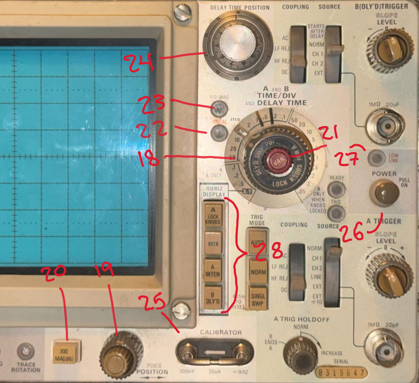
1. Controls time/div of A and B.

2. Fine/Position:

• Positions display horizontally for A sweep and B sweep.

1. X10 Mag:

• Increase displayed sweep rate by a factor of 10. Extend fastest sweep rate to 1 nanosecond/division. Magnified sweep is the center division of the unmagnified display.

1. Var:

• Provides continuously variable sweep rates between the calibrated setting of the A time/div switch.

1. UNCAL lamp:

• Indicated the A sweep rate is uncalibrated

1. X10 MAG lamp:

• Indicated that the X10 magnified is on

1. Delay time position:

• Provides variable sweep delay to more than 10 times the delay time indicated by the A time/div switch

1. Calibrator:

• A combination current loop/square wave voltage output that permits the operator to compensate voltage probes and check vertical gain, current probes, and oscilloscope operation.

1. Power

2. Low line lamp:

• Indicates the applied line voltage is below lower limit of the regulating range selected by the regulating range selector.

1. Horizontal Display:

• Determines the mode of operation for the horizontal deflection system.

Trigger

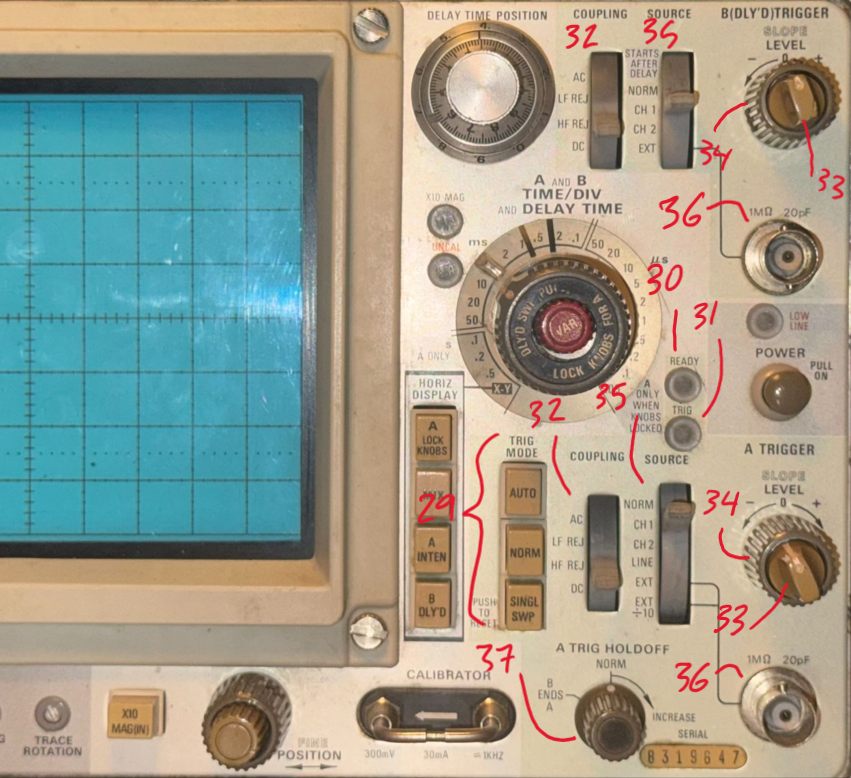
1. Trig Mode:

• Determines the mode of trigger operation for a sweep
  • Auto: Sweep is initiated by applied trigger signal, if trigger repetition is less than 20 hertz in the absence, sweep runs free with bright reference trace
  • Norm: Sweep is initiated by applied trigger signal, in absence of adequate trigger, there is no trace.
  • SINGL SWP: when pushbutton is pushed, A sweep operates in single sweep mode, after its displayed, further sweeps cannot be presented.

1. READY lamp:

• Indicated A sweep is “armed” and upon receipt of an adequate trigger, will present single-sweep display

1. TRIG lamp:

• Indicates A sweep is triggered and will produce stable display.

1. Coupling:

• Determines the method used to couple signals to trigger the generator circuit

  • AC: signals are capacitively coupled to input of the trigger circuit. Dc is rejected and signals below 50 kHz are attenuated.

  • LF REJ: signals are capacitively couple to the input of the trigger circuit. DC is rejected and signals below 30 Hz and above 50 kHz are attenuated.

  • DC: All components of a trigger signal are couple to the input of the trigger circuit.

1. Slope:

• Selects slop of the trigger signal that starts the sweep

  • +: sweep can be triggered from positive-going portion of a trigger signal

  • -: sweep can be triggered from the negative-going portion

• Correct slope setting is important in obtaining a display when only a portion of a cycle is being displayed

1. Level:

• Selects amplitude point on the trigger signal at which the sweep is triggered. It is usually adjusted for desired display after trigger source, coupling, and slop have been selected.

1. Source:

• Determines the source of the trigger signal coupled to the input of the trigger circuit.

1. External Trigger Inputs:

• Input connectors for external trigger signals

1. trig holdoff:

• Provides continuous control of time between sweeps, allows triggering on aperiodic signals. A sweep is reset at end of B sweep to provide fastest possible sweep repetition